Scientific Background
Blue Whale B-Call Vocalizations
Blue whale B calls are tonal harmonic signals typically 10–20 seconds in duration,
with a fundamental frequency that steps down between roughly 20 and 16 Hz. For
decades, these calls were thought to originate from Helmholtz resonance — air flowing
from the lungs into the upper respiratory spaces, with vocalization frequency
proportional to the size of the resonating organ.
A 2017 paper by Dziak et al. (Scientific Reports) proposed an alternative: blue
whales produce B calls by rapidly opening and closing respiratory valves (principally
the U-fold, homologous to vocal folds in terrestrial mammals), generating a series of
short-duration pneumatic air pulses. These pulses, taken together, produce the
fundamental frequency and overtone structure of the B call — analogous to how
repeating seismic or volcanic bursts generate harmonic tremor signals.
Key insight: The fundamental frequency and overtones are inversely
proportional to the time spacing between pulse peaks. Varying the inter-pulse
interval shifts the entire harmonic series up or down in frequency — which may be how
individual whales actively modulate their calls.
This model achieves a cross-correlation coefficient of r = 0.93 against real
hydrophone recordings of blue whale B calls at 55 m depth, outperforming sinusoidal
resonance models (r = 0.87).
Dziak, R. P., Haxel, J. H., Lau, T-K., Heimlich, S., Caplan-Auerbach, J., Mellinger, D. K.,
Matsumoto, H., & Mate, B. (2017). A pulsed-air model of blue whale B call vocalizations.
Scientific Reports, 7, 9122. DOI: 10.1038/s41598-017-09423-7
The Mathematics
Pulse Wavelet Construction
Each individual wavelet is constructed as the time derivative of a piecewise
Cauchy-like function q(t). The asymmetric shape — sharper on the leading edge,
slower decay on the trailing side — mimics the rapid valve opening and gradual
pressure release of a pneumatic pulse.
Pulse function — Equation (1)
P(t) = dq/dt
q(t) definition
q(t) = 1 / [(t − a)2 + 0.01] for t < a
q(t) = 10 / [(t − a)2 + 0.1] for t > a
Here a is a constant that sets the temporal location of the pulse peak,
keeping the duration under one second. In the model, a = 0.005, yielding
a pulse wavelet of approximately 0.068 seconds. Taking the derivative P(t) = dq/dt
produces the actual waveform shape:
Derivative P(t) — implemented form
P(t) = −2(t−a) / [(t−a)2 + 0.000001]2 for t < a
P(t) = −20(t−a) / [(t−a)2 + 0.000005]2 for t > a
A full synthetic B call is constructed by concatenating 99 repetitions of two
back-to-back pulses, then applying a sinusoidal volume envelope (sin 0→π/2 for
the attack half, sin π/2→π for the decay half). The final signal is scaled to
16-bit integer range and exported as a WAV file.
q(t)
Cauchy fn
→
P(t) = dq/dt
Wavelet
→
Truncate
500 samples
→
Repeat ×99
Pulse train
→
sin Envelope
Attack/Decay
→
Scale → i16
WAV out
Simulation Results
Python / NumPy — Waveform & Spectrogram
The plots below show (top) a single 0.068 s pulse wavelet, (middle) the full
synthesized waveform with sinusoidal amplitude envelope, and (bottom) the resulting
spectrogram. The harmonic structure — a fundamental and evenly spaced overtones —
is clearly visible, consistent with real blue whale B call recordings.
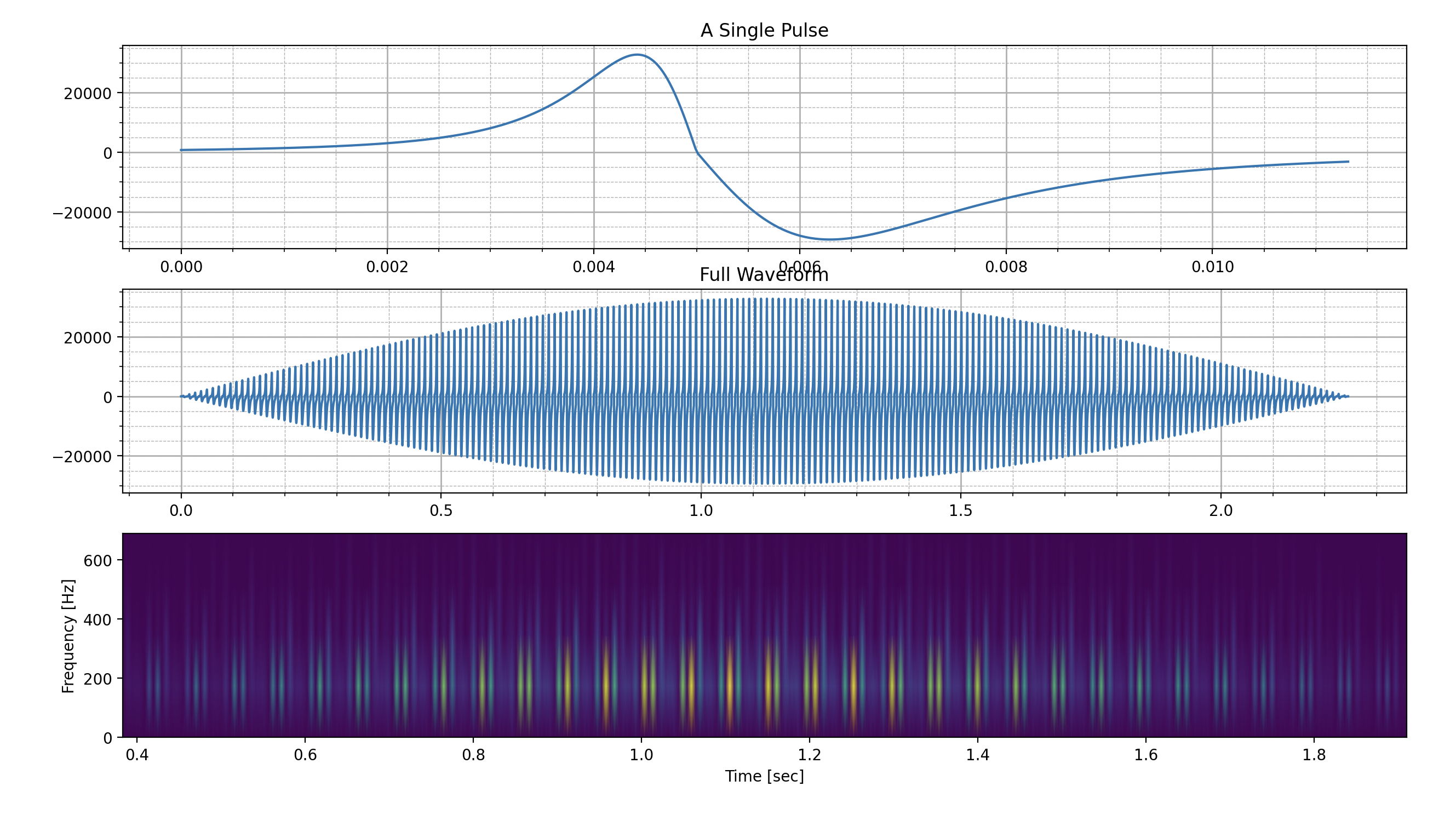
Notebook output — single pulse, full waveform, spectrogram
Interpretation: The spectrogram confirms harmonic content at integer
multiples of the fundamental, matching the 14.73 Hz fundamental and overtones
(29.5, 44.2, 58.9 Hz…) reported in the Dziak et al. paper. The envelope rise and fall
is visible in the amplitude modulation of the waveform.
Python Source
whale_script.py
The script below generates the whale song waveform, applies the sinusoidal volume
envelope, plots the single pulse, full waveform, and spectrogram, and writes the
output to a 16-bit WAV file (out.wav).
# Allows you to convert arrays into wav files to play audio
from scipy.io.wavfile import write
from scipy import signal
from scipy.fft import fftshift
import numpy as np
import matplotlib.pyplot as plt

p_duration = 0.068

samplerate = 44100
t_pulse = np.linspace(0, 1, samplerate)
a = 0.005

# Cauchy-like pulse function q(t)
q_t = np.array([(1/(((tp-a)**2) + 0.01)) if tp < a else (10/(((tp-a)**2) + 0.1)) for tp in t_pulse])

# Derivative of q_t — this is the actual pulse wavelet P(t)
QT = np.array([-2*((tp-a)/((((tp-a)**2)+0.000001))**2) if tp < a else -20*((tp-a)/((((tp-a)**2)+0.000005))**2) for tp in t_pulse])

# Scale the data to match the 16-bit min/max values of wav file
high = np.iinfo(np.int16).max
pulse_high = np.max(QT)

scale = high/pulse_high
QT_sc = QT[0:500]*scale

# String together a bunch of pulses to make a song
song = np.array([np.concatenate((QT_sc, QT_sc)) for x in range(1, 100)])
song = song.ravel()

t_song = np.arange(0, t_pulse[500]*198, 1/(samplerate))
print(np.size(t_song))
print(np.size(song))

# Create volume envelope for waveform based on sin function
sec_len = round(len(song)/4)
envelope_p1 = np.sin(np.linspace(0, np.pi/2, sec_len*2))
envelope_p2 = np.sin(np.linspace(np.pi/2, np.pi, sec_len*2 + (len(song) - sec_len*4)))
envelope_tot = np.concatenate((envelope_p1, envelope_p2))

# Apply the envelope to the song
final_song = np.array([song[i]*envelope_tot[i] for i in range(0, len(song))])

# Visualize the Spectrogram of the whale song
fs = samplerate
N = len(final_song)
f, t, Sxx = signal.spectrogram(final_song, fs)

# Visualize the waveforms (a single pulse and a song)
fig, ax = plt.subplots(3)

ax[0].plot(t_pulse[0:500], QT_sc)
ax[0].set_title("A Single Pulse")

ax[1].plot(t_song[0:np.size(song)], final_song)
ax[1].set_title("Full Waveform")

ax[0].minorticks_on()
ax[1].minorticks_on()
ax[0].grid(which='minor', linestyle='--', linewidth=0.5)
ax[0].grid(which='major', linestyle='-', linewidth=1)
ax[1].grid(which='minor', linestyle='--', linewidth=0.5)
ax[1].grid(which='major', linestyle='-', linewidth=1)

ax[2].pcolormesh(t, fftshift(f), fftshift(Sxx, axes=0), shading='gouraud')
ax[2].set_ylabel('Frequency [Hz]')
ax[2].set_xlabel('Time [sec]')

plt.show()

# Write output WAV file
out_f = 'out.wav'
write(out_f, samplerate, final_song.astype(np.dtype('i2')))
Reference
Primary Source
The pulse model and mathematical framework implemented in this project are drawn
directly from the following open-access paper:
Dziak, R. P., Haxel, J. H., Lau, T-K., Heimlich, S., Caplan-Auerbach, J.,
Mellinger, D. K., Matsumoto, H., & Mate, B. (2017).
A pulsed-air model of blue whale B call vocalizations.
Scientific Reports, 7, 9122.
doi: 10.1038/s41598-017-09423-7
— Published under Creative Commons Attribution 4.0 International License.